✖️ How to Add an “x” Suffix to Numbers in Excel — The Smartest Way to Format Multipliers

In financial models, product sheets, and business dashboards, it’s common to use an “x” to indicate multiplication factors — like 2.5x, 10x, or 0.8x. This small suffix quickly signals that the number represents a multiple — which is especially useful in pricing, valuation, or growth comparison contexts.

If you’re wondering why someone would format numbers this way, you might not work with Excel very often. But for someone who does this several times a day — like analysts, consultants, or product managers — repeating this formatting manually can become a tedious time drain and introduce inconsistencies.

This article presents three practical ways to add an “x” suffix to numbers in Excel — from traditional formatting options to a one-step solution using the QuickCel app.

1) Using the Ribbon

If you prefer a visual, menu-driven approach, you can apply a custom number format through Excel’s Ribbon.

✅ How it works:

1. Select the cells you want to format
2. Go to Home → Number Format dropdown → More Number Formats
3. In the Format Cells window, select Custom
4. Paste or type this format:
   • .##0,0x_);(#.##0,0x);@

⚠️ Drawbacks:

• Requires mouse interaction
• Slower for repeated use
• Not ideal for large datasets or high-frequency workflows
• Easy to forget the exact format string
• 🕒 Time required: ~10–15 seconds per selection

💡 If you only do this occasionally, this method might be enough for you — but it’s far from the most efficient solution.

2) Copying the Format from an Existing Cell

If you already have a properly formatted cell, you can use Excel’s Paste Special → Formats feature to copy the style to other cells.

✅ How it works:

1. Select a cell that has the correct formatting;
2. Press Ctrl + C;
3. Select the target cells
4. Use Paste Special by pressing Alt+H+V+R.

⚠️ Drawbacks:

• You must already have a pre-formatted cell
• Still involves multi-step navigation
• Not practical for repeated tasks
• Mouse or arrow-key navigation still needed
• 🕒 Time required: ~6–10 seconds per selection

3) Using QuickCel: One Shortcut, Zero Clicks

QuickCel introduces a faster, cleaner solution. With a single command — Ctrl + Shift + 8 — it instantly formats selected numbers to include an “x” suffix, applying the correct custom number format behind the scenes.

It also follows professional standards by displaying negative values in parentheses (e.g., (2.5x)), which is especially relevant in financial data, where negative numbers are commonly shown this way for clarity.

✅ How it works:

Ctrl + Shift + 8 → Apply multiplier format instantly

Before	Shortcut	After
2.5	Ctrl + Shift + 8	2.5x
-2.5	Ctrl + Shift + 8	(2.5x)
=A1+B1	Ctrl + Shift + 8	=A1+B1 (formatted as multiplier)

✅ Key Benefits:

• Execution time: ~0 seconds
• No mouse or navigation needed
• Works on both values and formulas
• Displays negative numbers in (parentheses) by default
• Keeps formatting consistent and professional
• Great for recurring tasks and high-volume data formatting
• Removes the need to remember format strings

4) What Else Can You Do with QuickCel?

QuickCel offers more than just number suffixes — it’s a complete toolkit to boost your productivity in Excel. Here are some of its most useful shortcuts:

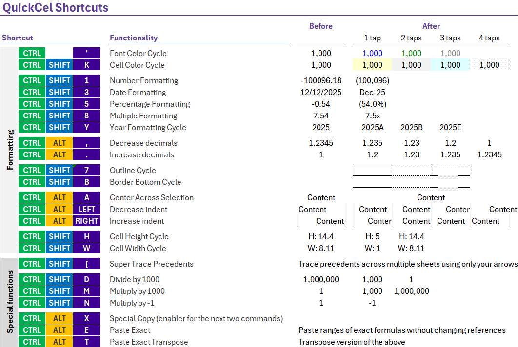
Each command is built to eliminate unnecessary clicks, reduce error-prone steps, and let you focus on actual analysis.

On average, QuickCel users save 100+ hours per year — the equivalent of more than two full workweeks — just by streamlining formatting and layout tasks.

5) Try It for Yourself

Whether you’re working with valuations, product comparisons, or marketing multipliers, QuickCel makes formatting multipliers instant and consistent.

Learn all about QuickCel’s features on our website: www.quickcel.software

Learn all about QuickCel’s features on our website: www.quickcel.software 👉 Download QuickCel and discover how one shortcut can transform your workflow.