Working with percentages in Excel is common when calculating growth rates, survey results, budget deviations, or performance metrics. Whether you’re building dashboards, analyzing campaign performance, or formatting KPI tables, applying percentage formatting makes your data easier to understand and communicate.
You might be wondering, “Why do I need a shortcut to turn a number into a percentage? It’s so simple – it’s right on the first page of the menu.” But if you work with negative percentages and want to follow financial modeling standards, you’ll need those values to appear in parentheses – and the default menu button won’t help you with that.
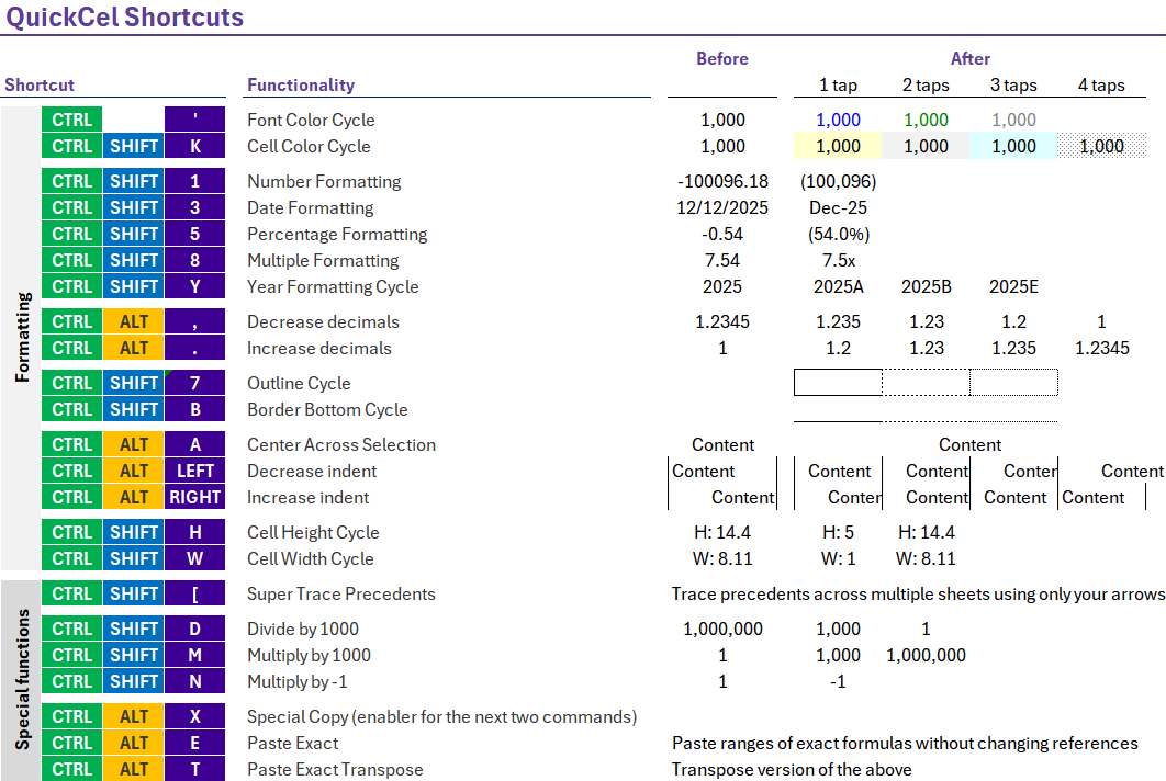
In this article, we’ll explore the traditional methods to format numbers as percentages – and show you how to do it in one keystroke using QuickCel’s Ctrl + Shift + 5 shortcut. Not only is it faster – it applies the correct formatting standard automatically, keeping your spreadsheets clean and professional.
1) Using the Number Formatting Menu
The classic way to format numbers as percentages is through the Number Format options in the Ribbon.
✅ How it works:
- Select the cell or range of numbers
- Go to Home → Number group
- Click the dropdown menu
- Choose More Number Formats at the bottom
- Under Custom, type or select:
- .##0%_);(#.##0%);@
⚠️ Drawbacks:
- Requires multiple clicks and navigation
- Doesn’t automatically apply parentheses to negative values unless you enter the custom format manually
- Easy to forget or misapply the correct pattern
- Slows down repeated formatting tasks
- 🕒 Execution Time: 5–7 seconds per change
💡 This method may be enough if you only format percentages occasionally – but not ideal for high-volume formatting or reports requiring accuracy.
2) Copying the Formatting from an Existing Cell
If you already have a cell with the proper percentage formatting – including negative values in parentheses – you can reuse it across your sheet.
✅ How it works:
- Select a cell already formatted with: .##0%_);(#.##0%);@
- Press Ctrl + C
- Select the target cells
- Use Paste Special using the shortcut Alt+H+V+R.
⚠️ Drawbacks:
- Requires an existing, correctly formatted cell
- You still need to manually configure it the first time
- Easy to overwrite other formats unintentionally
- Not scalable if you’re switching between styles often
- 🕒 Execution Time: 3–5 seconds (if you have a reference cell)
3) Using QuickCel: Format Percentages Instantly
With QuickCel, formatting numbers as percentages becomes instant and professional. Just press Ctrl + Shift + 5, and it automatically applies the standard financial format.
This format ensures:
- Positive numbers show as 12.3%
- Negative numbers show as (12.3%) – instead of with a minus sign
- Decimal place is included for clarity
✅ How it works:
| Original Value | Shortcut Pressed | Resulting Format |
| 0.123 | Ctrl + Shift + 5 | 12.3% |
| -0.123 | Ctrl + Shift + 5 | (12.3%) |
| 0.5 | Ctrl + Shift + 5 | 50.0% |
✅ Key Benefits:
- No need to open any menus or remember custom patterns
- Automatically formats negative percentages in parentheses
- Applies decimal precision consistently
- 100% keyboard-driven — no mouse required
- Ideal for financial models, dashboards, and recurring reports
- 🕒 Execution Time: ~0 seconds — instant
4) What Else Can You Do with QuickCel?
QuickCel offers dozens of powerful formatting shortcuts designed for professionals who want to save time and reduce manual work in Excel.
🔁 On average, QuickCel users save 100+ hours per year by replacing manual steps with powerful keyboard shortcuts.
5) Try It for Yourself
If you’re still formatting percentages manually – or struggling to get negative values to display properly – it’s time to simplify your workflow. Use Ctrl + Shift + 5 with QuickCel and never worry about formatting mistakes again.
🌐 Learn more: www.quickcel.software
⬇️ Download QuickCel for free and streamline every step of your Excel workflow.