When working with numbers in Excel, presentation matters. Whether you’re dealing with large sums of money, quantities, or any other numerical data, a clear, consistent format makes your information easier to read and understand. One of the most common number formats used across many industries – especially in finance – includes a thousands separator, parentheses for negative values, and dashes for zero values.
If you’re wondering why someone would need a shortcut for this, you probably don’t use Excel that often – or maybe your work doesn’t require this kind of formatting. But this format is quite common in the financial market, and if you need to apply it repeatedly, doing it manually can consume a lot of time – time that could be better spent refining other parts of your analysis.
In this article, we’ll walk you through the traditional methods to apply this format and show you how QuickCel makes it lightning-fast with a single keystroke.
1) Using the Ribbon Menu
Most users apply number formatting by going to the Home tab in Excel and manually adjusting settings in the Format Cells dialog. While this works, applying a financial-style format – with commas, parentheses, and dashes – requires several steps.
✅ How it works:
- Select the cells you want to format
- Go to Home → Number section
- Click the small Format Cells launcher icon (or right-click > Format Cells)
- Choose Custom
- Enter the following format: #.##0;(#.##0);-;@
This format:
- Adds commas for thousands (e.g., 1,000)
- Displays negative numbers in parentheses (e.g., (500))
- Shows a dash for zero values instead of 0
💡 Tip: This method might be enough if you only make this formatting adjustment occasionally.
⚠️ Drawbacks:
- Time-consuming for large datasets
- Requires mouse navigation and manual entry
- Easy to forget or mistype the formatting code
- Not efficient for repeated use
- 🕒 Execution Time: 5–7 seconds per change
2) Copying the Format from an Existing Cell
If you already have a properly formatted cell, you can use Excel’s Paste Special → Formats feature to copy the style to other cells.
✅ How it works:
- Select a cell that has the correct formatting
- Press Ctrl + C
- Select the target cells
- Press Alt + H + V + R
⚠️ Drawbacks:
- You must already have a pre-formatted cell
- You still need to create that cell the first time
- Not scalable for multiple formatting styles across sheets
- 🕒 Execution Time: 3–5 seconds per change
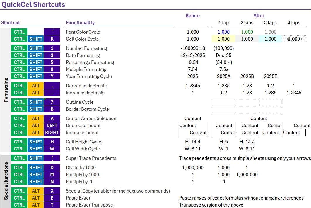
3) Using QuickCel: Format Instantly with One Shortcut
With QuickCel, you can apply the correct number formatting instantly using the Ctrl + Shift + 1 shortcut. This applies the custom format: #.##0;(#.##0);-;@
✅ What it does:
- Adds thousands separators (commas)
- Displays negative numbers in parentheses
- Replaces zeros with dashes
- Maintains clean alignment for reporting
📊 Example Table:
| Input | Ctrl + Shift + 1 | Displayed As |
| 1000 | ✅ | 1,000 |
| -500 | ✅ | (500) |
| 0 | ✅ | – |
| 3200000 | ✅ | 3,200,000 |
✅ Key Benefits:
- No need to open menus or type formatting codes
- Keeps your workflow keyboard-driven
- Perfect for financial reports and large data sets
- Applies professional formatting instantly
- Works seamlessly with thousands of values at once
- 🕒 Execution Time: ~0 seconds (instant toggle)
4) What Else Can You Do with QuickCel?
QuickCel offers dozens of formatting, layout, and navigation shortcuts to help you clean up spreadsheets without touching your mouse.
⚡ QuickCel users save over 100 hours per year – eliminating tedious formatting steps and allowing more time for data modeling, insights, and analysis.
5) Try It for Yourself
Ready to upgrade your number formatting workflow in Excel?
Use Ctrl + Shift + 1 to instantly apply professional-grade formatting to your data – and focus more on what matters most.
🌐 Learn more at: www.quickcel.software
⬇️ Download QuickCel for free and make formatting one less thing to worry about.